Preliminaries

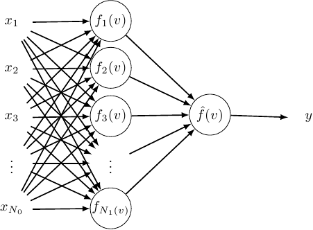
The backpropagation is one of the most popular method of training multilayered artificial neural networks - ANN. ANN classify data, and can be thought of as function approximators. A multilayer ANN can approximate any continuous function.

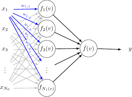
A two-layered fully-connected ANN can look like this:

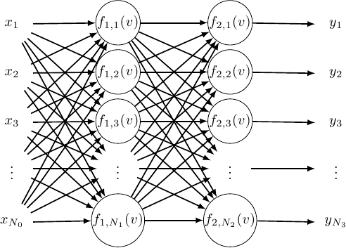
Where \(f_{A,B}\) are individual neurons. A neuron can have multiple weighted inputs, and connects to other neurons in the next layer. Additionally we add some bias – a value that doesn’t depend on the neurons injut. Here you can see a schematic representation of a single neuron.

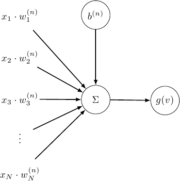
The \(b^{(n)}\) here is our bias value, and \(g(v)\) is a function called the activation function. Thus, the output of a single neuron \(f_{A,B}(v) = g \left ( \left ( \displaystyle \sum \limits_{i = 0}^N x_i \cdot w^{(A,B)}_i \right ) + b^{(A,B)} \right)\).

The simplest activation function is the identity function. When using a threshold activation function a single neuron divides the space into two parts – a single neuron with a threshold activation is a primitive classifier.

A single neuron can only separate the space using a single plane/line – the two data classes must be linearly separable.

Using two layers, and a nonlinear activation function is what makes a multilayered neural network work – it let’s us map an vector from \(\mathbb{R}^N\) and contract/expand it into \(\mathbb{R}^{N'}\) where it now is (hopefully) linearly separable.

The output of our hypothetical network is calculated as:

\[y_n = f_{2,n}(v) = g \left( \displaystyle \sum \limits_{i = 1}^{N_1} f_{1,i}(v) \cdot w_{f_{1, i} - f_{2, n}} + b_{2, n} \right)\]

Where \(f_{1, i}(v)\) is the output of the \(i\)-th first layer neuron:

\[f_{1, i}(v) = g \left( \displaystyle \sum \limits_{j = 1}^{N_0} x_j \cdot w_{x_{j} - f_{1, i}} + b_{1, i} \right )\]

\(w_{A - B}\) is the weight between nodes \(A\) and \(B\), and \(b_{i,j}\) is the bias of the \(j\)-th neuron in the \(i\)-th layer.

Training

Lets suppose, you want to teach this network - it has \(N_0\) inputs, and \(N_3\) outputs. To teach the network you must provide a teacher set \(t\) with \(M\) samples. The teacher set consists of known correct input/output values.

Training the network should minimize the difference between the correct outputs in the teacher set, and the output of the network. We will try to minimize the root mean square (RMS) error.

The only thing that determines the output is the weights between the nodes of the network so the error will be a function of the weights:

\[E(w_{A - B}) = \frac{1}{2} \displaystyle \sum \limits_{i = 1}^{M} \left( y_n^{(i)} - t^{(i)}_n \right)^2\]

Where \(y_n^{(i)}\) is the \(i\)-th output of the \(n\)-th output neuron. Using this definition of error we will derive the backpropagation formula for batch learning (on-line learning would be without the sum over every sample). The \(\frac{1}{2}\) term will come in handy during derivation.

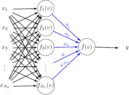
To simplify bookkeeping a little we will switch to a simplified network with only one output. Because the weights between the hidden layer and output layer don’t depend on each other we can do that without any loss of generality.

The weights between the input layer and hidden layer will be labeled as follows:

And the weights between the hidden and output layer are simply:

Because we have one output the error can now be simplified as:

\[E(w) = \frac{1}{2} \displaystyle \sum \limits_{i = 1}^{M} \left( y^{(i)} - t^{(i)} \right)^2\]

To minimize the error we will update the weights of the network so that the expected error in the next iteration will be lower (gradient descent).

\[w{(l + 1)} = w^{(l)} - h \cdot \nabla E(w^{(l)})\]

Where \(l\) is the iteration “counter”, and \(h\) is a learning rate \(0 < h \le 1\).

Deriving the formula

Hidden layer – output layer

The weight update formula for \(\hat{w_1}\) is: \(\hat{w}_1^{(l + 1)} = \hat{w}_1^{(l)} - h \cdot \nabla E(\hat{w}_1^{(l)})\)

The error:

\[\displaystyle E(\hat{w}_1^{(l)}) = \frac{1}{2} \sum \limits_{i = 1}^{M} \left( y^{(i)} - t^{(i)} \right)^2\]

So lets proceed to derivate the error function.

\[\displaystyle \nabla E(\hat{w}_1^{(l)}) = \frac{\partial}{\partial \hat{w}_1^{(l)}} \frac{1}{2} \sum \limits_{i = 1}^{M} \left( y^{(i)} - t^{(i)} \right)^2\]

Lets skip writing out the iteration index \(l\) to clear it a bit.

\[\displaystyle \nabla E(\hat{w}_1) = \frac{\partial}{\partial \hat{w}_1} \frac{1}{2} \sum \limits_{i = 1}^{M} \left( y^{(i)} - t^{(i)} \right)^2\]

Using the chain rule:

\[\displaystyle \frac{\partial}{\partial \hat{w}_1} \frac{1}{2} \sum \limits_{i = 1}^{M} \left( y^{(i)} - t^{(i)} \right)^2 = \frac{1}{2} \sum \limits_{i = 1}^{M} 2 \left( y^{(i)} - t^{(i)} \right) \frac{\partial}{\partial \hat{w}_1} \left( y^{(i)} - t^{(i)} \right)\]

The \(\frac{1}{2}\) and \(2\) terms cancel each other out leaving:

\[\displaystyle \nabla E(\hat{w}_1) = \sum \limits_{i = 1}^{M} \left( y^{(i)} - t^{(i)} \right) \frac{\partial}{\partial \hat{w}_1} \left( y^{(i)} - t^{(i)} \right)\]

The known outputs \(y^{(i)}\) don’t depend on the input weights, and are essentially constants. W.r.t \(w_1\) their derivative is zero, leaving:

\[\displaystyle \nabla E(\hat{w}_1) = \sum \limits_{i = 1}^{M} \left( y^{(i)} - t^{(i)} \right) \frac{\partial}{\partial \hat{w}_1} y^{(i)} =\] \[\displaystyle \sum \limits_{i = 1}^{M} \left( y^{(i)} - t^{(i)} \right) \frac{\partial}{\partial \hat{w}_1} g(\hat{r}^{(i)})\]

Where \(\hat{r}\) is the input to the output layer neuron, \(\hat{r}^{(i)}\) is the neuron input (what goes to the activation function) with respect to the \(i\)-th training input. \(r_j\) will be the input of the \(j\)-th neuron in the hidden layer:

\[\displaystyle \nabla E(\hat{w}_1) = \sum \limits_{i = 1}^{M} \left( y^{(i)} - t^{(i)} \right) \frac{\partial}{\partial \hat{w}_1} g \left( \left( \sum \limits_{j = 1}^{N_1} g_{j}(r_j^{(i)}) \cdot \hat{w_j} \right) + \hat{b} \right)\]

Where \(\hat{b}\) is the bias of the output neuron. If we use the chain rule once again we will have:

\[\displaystyle \nabla E(\hat{w}_1) = \sum \limits_{i = 1}^{M} \left( y^{(i)} - t^{(i)} \right) g'(\hat{r}^{(i)}) \cdot \frac{\partial}{\partial \hat{w}_1} \left( \left( \sum \limits_{j = 1}^{N_1} g_{j}(r_j^{(i)}) \cdot \hat{w_i} \right) + \hat{b} \right)\]

Clearly, the only term in the expression \(\displaystyle \left( \sum \limits_{j = 1}^{N_1} g_{i}(v) \cdot \hat{w_i} \right) + \hat{b}\) that depends on \(\hat{w}_1\) is \(f_1(r^{(i)}_1) \cdot w_1\). The rest of the sum will zero out after derivation. Therefore, we arrive at:

\[\displaystyle \nabla E(\hat{w}_1) = \sum \limits_{i = 1}^{M} \left( y^{(i)} - t^{(i)} \right) g'(\hat{r}^{(i)}) \cdot \frac{\partial}{\partial \hat{w}_1} \left( \left( g(r_1^{(i)}) \cdot \hat{w_1} \right) + \hat{b} \right) =\] \[\displaystyle \sum \limits_{i = 1}^{M} \left( y^{(i)} - t^{(i)} \right) g'(\hat{r}^{(i)}) \cdot g(r_1^{(i)})\]

And the full formula for the weight update:

\[\displaystyle \hat{w}_1^{(l + 1)} = w_1^{(l)} - h \cdot \sum \limits_{i = 1}^{M} \left( y^{(i)} - t^{(i)} \right) g'(\hat{r}^{(i)}) \cdot g(r_1^{(i)})\]

Derivations of \(\displaystyle \hat{w}_2 \ldots \hat{w}_{N_1}\) are similar and I’ll leave them out.

Input layer – hidden layer

Most of this derivation will be similar to output layer case written before, I’ll start commenting when we’ll get to the differences. I’ll only do the deriviation for \(w_{1,1}\), others can be done in a similar fashion.

\[\displaystyle w_{1, 1}^{(l + 1)} = w_{1,1}^{(l)} - h \cdot \nabla E(w_{1, 1}^{(l)})\] \[\displaystyle E(w_{1,1}^{(l)}) = \frac{1}{2} \sum \limits_{i = 1}^{M} \left( y^{(i)} - t^{(i)} \right)^2\] \[\displaystyle \nabla E(w_{1,1}^{(l)}) = \frac{\partial}{\partial w_{1,1}^{(l)}} \frac{1}{2} \sum \limits_{i = 1}^{M} \left( y^{(i)} - t^{(i)} \right)^2\]

Lets drop the unwieldy indices as before and continue:

\[\displaystyle \frac{\partial}{\partial w_{1,1}} \frac{1}{2} \sum \limits_{i = 1}^{M} \left( y^{(i)} - t^{(i)} \right)^2 = \frac{1}{2} \sum \limits_{i = 1}^{M} 2 \left( y^{(i)} - t^{(i)} \right) \frac{\partial}{\partial w_{1,1}} \left( y^{(i)} - t^{(i)} \right) =\] \[\displaystyle \frac{1}{2} \sum \limits_{i = 1}^{M} \left( y^{(i)} - t^{(i)} \right) \frac{\partial}{\partial w_{1,1}} \left( y^{(i)} - t^{(i)} \right) =\] \[\displaystyle \sum \limits_{i = 1}^{M} \left( y^{(i)} - t^{(i)} \right) \frac{\partial}{\partial w_{1,1}} y^{(i)} =\] \[\displaystyle \sum \limits_{i = 1}^{M} \left( y^{(i)} - t^{(i)} \right) \frac{\partial}{\partial w_{1,1}} g(\hat{r}^{(i)})\]

Here, it gets interesting, we must find the derivate of \(\displaystyle g(\hat{r}^{(i)})\) w.r.t \(w_{1, 1}\).

\[\displaystyle \nabla E \left (w_{1,1} \right ) = \sum \limits_{i = 1}^{M} \left( y^{(i)} - t^{(i)} \right) \frac{\partial}{\partial w_{1,1}} g(\hat{r}^{(i)}) =\] \[\displaystyle \sum \limits_{i = 1}^{M} \left( y^{(i)} - t^{(i)} \right) \frac{\partial}{\partial w_{1,1}} g \left( \left( \sum \limits_{j = 1}^{N_1} g(r_j^{(i)}) \cdot \hat{w_j} \right) + \hat{b} \right)\]

Using the chain rule:

\[\nabla E \left (w_{1,1} \right ) = \sum \limits_{i = 1}^{M} \left( y^{(i)} - t^{(i)} \right) g'(\hat{r}^{(i)}) \cdot \frac{\partial}{\partial w_{1,1}} \left( \left( \sum \limits_{j = 1}^{N_1} g(r_j^{(i)}) \cdot \hat{w_j} \right) + \hat{b} \right) =\] \[\displaystyle \sum \limits_{i = 1}^{M} \left( y^{(i)} - t^{(i)} \right) g'(\hat{r}^{(i)}) \cdot \frac{\partial}{\partial w_{1,1}} \left( \sum \limits_{j = 1}^{N_1} g(r_j^{(i)}) \cdot \hat{w_j} \right) + \frac{\partial}{\partial w_{1,1}} \hat{b} =\] \[\displaystyle \sum \limits_{i = 1}^{M} \left( y^{(i)} - t^{(i)} \right) g'(\hat{r}^{(i)}) \cdot \frac{\partial}{\partial w_{1,1}} \left( \sum \limits_{j = 1}^{N_1} g(r_j^{(i)}) \cdot \hat{w_j} \right)\]

The only part of the sum \(\displaystyle \sum \limits_{j = 1}^{N_1} g(r_j^{(i)}) \cdot \hat{w_j}\) that depends on \(w_{1, 1}\) is \(\displaystyle g(r_1^{(i)}) \cdot \hat{w_1}\), continuing:

\[\displaystyle \nabla E \left (w_{1,1} \right ) = \sum \limits_{i = 1}^{M} \left( y^{(i)} - t^{(i)} \right) g'(\hat{r}^{(i)}) \cdot \frac{\partial}{\partial w_{1,1}} \left( g(r_1^{(i)}) \cdot \hat{w_1} \right) =\] \[\displaystyle \sum \limits_{i = 1}^{M} \left( y^{(i)} - t^{(i)} \right) g'( \hat{r}^{(i)}) \cdot \hat{w_1} \cdot \frac{\partial}{\partial w_{1,1}} g(r_1^{(i)}) =\] \[\displaystyle \sum \limits_{i = 1}^{M} \left( y^{(i)} - t^{(i)} \right) g'( \hat{r}^{(i)}) \cdot \hat{w_1} \cdot \frac{\partial}{\partial w_{1,1}} g \left( \left( \sum \limits_{j = 1}^{N_0} x_{j}^{(i)} \cdot w_{1, j} \right ) + b_1 \right )\]

Using the chain rule:

\[\displaystyle \nabla E \left (w_{1,1} \right ) =\] \[\displaystyle \sum \limits_{i = 1}^{M} \left( y^{(i)} - t^{(i)} \right) g'(\hat{r}^{(i)}) \cdot \hat{w_1} \cdot g'(r_1^{(i)}) \cdot \frac{\partial}{\partial w_{1,1}} \left( \left( \sum \limits_{j = 1}^{N_0} x_{j}^{(i)} \cdot w_{1, j} \right ) + b_1 \right ) =\] \[\displaystyle \sum \limits_{i = 1}^{M} \left( y^{(i)} - t^{(i)} \right) g'(\hat{r}^{(i)}) \cdot \hat{w_1} \cdot g'(r_1^{(i)}) \cdot \frac{\partial}{\partial w_{1,1}} \sum \limits_{j = 1}^{N_0} x_{j}^{(i)} \cdot w_{1, j} + \frac{\partial}{\partial w_{1,1}} b_1 =\] \[\displaystyle \sum \limits_{i = 1}^{M} \left( y^{(i)} - t^{(i)} \right) g'(\hat{r}^{(i)}) \cdot \hat{w_1} \cdot g'(r_1^{(i)}) \cdot \frac{\partial}{\partial w_{1,1}} \sum \limits_{j = 1}^{N_0} x_{j}^{(i)} \cdot w_{1, j}\]

In the sum: \(\displaystyle \sum \limits_{j = 1}^{N_0} x_{j}^{(i)} \cdot w_{1, j}\) the only term with a non-zero derivative w.r.t \(w_{1, 1}\) is \(x_1^{(i)} \cdot w_{1, 1}\)

\[\displaystyle \nabla E \left (w_{1,1} \right ) = \sum \limits_{i = 1}^{M} \left( y^{(i)} - t^{(i)} \right) g'(\hat{r}^{(i)}) \cdot \hat{w_1} \cdot g'(r_1^{(i)}) \cdot \frac{\partial}{\partial w_{1,1}} \left( x_1^{(i)} \cdot w_{1_, 1} \right) =\] \[\displaystyle \nabla E \left (w_{1,1} \right ) = \sum \limits_{i = 1}^{M} \left( y^{(i)} - t^{(i)} \right) g'(\hat{r}^{(i)}) \cdot \hat{w_1} \cdot g'(r_1^{(i)}) \cdot x_1^{(i)}\]

Finally, the weight update rule for the hidden layer:

\[\displaystyle w_{1, 1}^{(l + 1)} = w_{1, 1}^{(l)} - h \cdot \sum \limits_{i = 1}^{M} \left( y^{(i)} - t^{(i)} \right) g'(\hat{r}^{(i)}) \cdot \hat{w_1} \cdot g'(r_1^{(i)}) \cdot x_1^{(i)}\]

Biases

Derving biases of neurons is mostly the same as regular weights, the only difference is in a couple of last steps:

\[\displaystyle \nabla E(\hat{b}) = \sum \limits_{i = 1}^{M} \left( y^{(i)} - t^{(i)} \right) g'(\hat{r}^{(i)}) \cdot \frac{\partial}{\partial \hat{b}} \left( \left( \sum \limits_{j = 1}^{N_1} g(r_j^{(i)}) \cdot \hat{w_i} \right) + \hat{b} \right) =\] \[\displaystyle \nabla E(\hat{b}) = \sum \limits_{i = 1}^{M} \left( y^{(i)} - t^{(i)} \right) g'(\hat{r}^{(i)}) \cdot \frac{\partial}{\partial \hat{b}} \left( \sum \limits_{j = 1}^{N_1} g(r_j^{(i)}) \cdot \hat{w_i} \right) + \frac{\partial}{\partial \hat{b}} \hat{b} =\] \[\displaystyle \nabla E(\hat{b}) = \sum \limits_{i = 1}^{M} \left( y^{(i)} - t^{(i)} \right) g'(\hat{r}^{(i)}) \cdot \frac{\partial}{\partial \hat{b}} \hat{b} =\] \[\displaystyle \nabla E(\hat{b}) = \sum \limits_{i = 1}^{M} \left( y^{(i)} - t^{(i)} \right) g'(\hat{r}^{(i)})\]

Similarly, for the hidden layer:

\[\displaystyle \nabla E \left (b_{1} \right ) =\] \[\displaystyle \sum \limits_{i = 1}^{M} \left( y^{(i)} - t^{(i)} \right) g'(\hat{r}^{(i)}) \cdot \hat{w_1} \cdot g'(r_1^{(i)}) \cdot \frac{\partial}{\partial b_{1}} \left( \left( \sum \limits_{j = 1}^{N_0} x_{j}^{(i)} \cdot w_{1, j} \right ) + b_1 \right ) =\] \[\displaystyle \sum \limits_{i = 1}^{M} \left( y^{(i)} - t^{(i)} \right) g'(\hat{r}^{(i)}) \cdot \hat{w_1} \cdot g'(r_1^{(i)})\]

Putting it all together

To sum up all we’ve done so far, the weight update rules for the output layer:

\[\displaystyle \forall A \in 1 \ldots N_1:\] \[\displaystyle \hat{w}_A^{(l + 1)} = w_A^{(l)} - h \cdot \sum \limits_{i = 1}^{M} \left( y^{(i)} - t^{(i)} \right) g'(\hat{r}) \cdot g(r_A^{(i)})\]

And for the hidden layer:

\[\displaystyle \forall A \in 1 \ldots N_0, \forall B \in 1 \ldots N_1:\] \[\displaystyle w_{A, B}^{(l + 1)} = w_{A, B}^{(l)} - h \cdot \sum \limits_{i = 1}^{M} \left( y^{(i)} - t^{(i)} \right) g'(\hat{r}^{(i)}) \cdot \hat{w_B} \cdot g'(r_B^{(i)}) \cdot x_A^{(i)}\]

And finally, biases:

\[\displaystyle \hat{b}^{(l + 1)} = \hat{b}^{(l)} - h \cdot \sum \limits_{i = 1}^{M} \left( y^{(i)} - t^{(i)} \right) g'(\hat{r}^{(i)})\] \[\displaystyle \forall B \in 1 \ldots N_0\] \[\displaystyle b_B^{(l + 1)} = b_B^{(l)} - h \cdot \sum \limits_{i = 1}^{M} \left( y^{(i)} - t^{(i)} \right) g'(\hat{r}^{(i)}) \cdot \hat{w_B} \cdot g'(r_B^{(i)})\]

Why backpropagation?

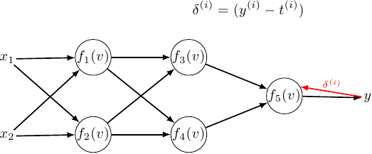
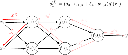
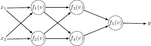
Why the weight update algorithm is called the backpropagation algorithm may not be so apparent when considering the usual case of a network with two layers. For it to become more obvious, we will consider a simple network with three layers:

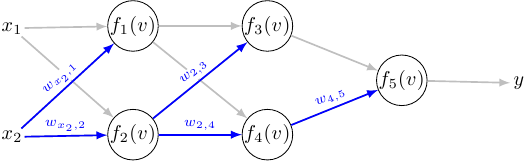
The weight update for the output layer is similar as before:

\[\displaystyle w_{3,5}^{(l + 1)} = w_{3,5}^{(l)} - h \cdot \sum \limits_{i = 1}^{M} \left( y^{(i)} - t^{(i)} \right) g'(r_5) \cdot g(r_3^{(i)})\] \[\displaystyle w_{4,5}^{(l + 1)} = w_{3,5}^{(l)} - h \cdot \sum \limits_{i = 1}^{M} \left( y^{(i)} - t^{(i)} \right) g'(r_5) \cdot g(r_4^{(i)})\]

For second hidden layer:

\[\displaystyle w_{1,3}^{(l + 1)} = w_{1,3}^{(l)} - h \cdot \sum \limits_{i = 1}^{M} \left( y^{(i)} - t^{(i)} \right) g'(r_5) w_{3,5} \cdot g'(r_3) \cdot g(r_1)\] \[\displaystyle w_{1,4}^{(l + 1)} = w_{1,4}^{(l)} - h \cdot \sum \limits_{i = 1}^{M} \left( y^{(i)} - t^{(i)} \right) g'(r_5) w_{4,5} \cdot g'(r_4) \cdot g(r_1)\] \[\displaystyle w_{2,3}^{(l + 1)} = w_{2,3}^{(l)} - h \cdot \sum \limits_{i = 1}^{M} \left( y^{(i)} - t^{(i)} \right) g'(r_5) w_{3,5} \cdot g'(r_3) \cdot g(r_2)\] \[\displaystyle w_{2,4}^{(l + 1)} = w_{2,4}^{(l)} - h \cdot \sum \limits_{i = 1}^{M} \left( y^{(i)} - t^{(i)} \right) g'(r_5) w_{4,5} \cdot g'(r_4) \cdot g(r_2)\]

Weight update for the first hidden layer

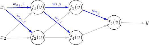
Things start to be interesting in the first hidden layer: let’s analyze the weight update for \(w_{x_1,1}\):

\[\displaystyle \nabla E \left (w_{x_1,1} \right ) = \sum \limits_{i = 1}^{M} \left( y^{(i)} - t^{(i)} \right) \frac{\partial}{\partial w_{x_1,1}} g(r_5^{(i)}) =\] \[\displaystyle \sum \limits_{i = 1}^{M} \left( y^{(i)} - t^{(i)} \right) g'(r_5^{(i)}) \frac{\partial}{\partial w_{x_1,1}} r_5^{(i)} =\] \[\displaystyle \sum \limits_{i = 1}^{M} \left( y^{(i)} - t^{(i)} \right) g'(r_5) \frac{\partial}{\partial w_{x_1,1}} \left( w_{3,5} g(r_3^{(i)}) + w_{4,5} g(r_4^{(i)}) + b_5 \right) =\]

I’ll do the relevant partials separately:

The derivative of the bias is, of course, zero:

\[\displaystyle \frac{\partial}{\partial w_{x_1,1}} b_5 = 0\]

The first term:

\[\displaystyle \frac{\partial}{\partial w_{x_1,1}} \left( w_{3,5} g(r_3^{(i)}) \right) =\] \[\displaystyle w_{3,5} \cdot \frac{\partial}{\partial w_{x_1,1}} g(r_3^{(i)}) =\] \[\displaystyle w_{3,5} \cdot g'(r_3^{(i)}) \frac{\partial}{\partial w_{x_1,1}} r_3^{(i)} =\] \[\displaystyle w_{3,5} \cdot g'(r_3^{(i)}) \frac{\partial}{\partial w_{x_1,1}} \left( w_{1,3} \cdot g(r_1^{(i)}) + w_{2,3} \cdot g(r_2^{(i)}) + b_3 \right)\]

The deriative of \(b_3\) and output of the \(2\)-nd neuron are 0 w.r.t \(w_{x_1,1}\), so:

\[\displaystyle \frac{\partial}{\partial w_{x_1,1}} \left( w_{3,5} g(r_3)^{(i)} \right) = w_{3,5} \cdot g'(r_3^{(i)}) \frac{\partial}{\partial w_{x_1,1}} \left( w_{1,3} \cdot g(r_1^{(i)}) \right) =\] \[\displaystyle w_{3,5} \cdot g'(r_3^{(i)}) \cdot w_{1,3} \cdot g'(r_1^{(i)}) \frac{\partial}{\partial w_{x_1,1}} r_1^{(i)} =\] \[\displaystyle w_{3,5} \cdot g'(r_3^{(i)}) w_{1,3} \cdot g'(r_1^{(i)}) \frac{\partial}{\partial w_{x_1,1}} \left( w_{x_1,1} x_1^{(i)} + w_{x_2,1} x_2^{(i)} + b_1 \right) =\] \[\displaystyle w_{3,5} \cdot g'(r_3^{(i)}) w_{1,3} \cdot g'(r_1^{(i)}) \cdot x_1^{(i)}\]

The second part is:

\[\displaystyle \frac{\partial}{\partial w_{x_1,1}} \left( w_{4,5} g(r_4)^{(i)} \right) = w_{4,5} \cdot g'(r_4^{(i)}) w_{1,4} \cdot g'(r_1^{(i)}) \cdot x_1^{(i)}\]

Putting it toghether we get:

\[\displaystyle \nabla E \left (w_{x_1,1} \right ) =\] \[\displaystyle \sum \limits_{i = 1}^{M} \left( y^{(i)} - t^{(i)} \right) g'(r_5) \cdot g'(r_1^{(i)}) \cdot x_1^{(i)} \left( w_{3,5} \cdot g'(r_3^{(i)}) w_{1,3} + w_{4,5} \cdot g'(r_4^{(i)}) w_{1,4} \right)\]

Error signal

The \((y^{(i)} - t^{(i)})\) term is sometimes written as \(\delta^{(i)}\) and is called the error signal. If we rewrite the weight update rules for the output layer to use it we will get:

\[\displaystyle w_{3,5}^{(l + 1)} = w_{3,5}^{(l)} - h \cdot \sum \limits_{i = 1}^{M} \delta^{(i)} \cdot g'(r_5) \cdot g(r_3^{(i)})\] \[\displaystyle w_{4,5}^{(l + 1)} = w_{3,5}^{(l)} - h \cdot \sum \limits_{i = 1}^{M} \delta^{(i)} \cdot g'(r_5) \cdot g(r_4^{(i)})\]

For the second hidden layer:

\[\displaystyle w_{1,3}^{(l + 1)} = w_{1,3}^{(l)} - h \cdot \sum \limits_{i = 1}^{M} \delta^{(i)} \cdot g'(r_5) w_{3,5} \cdot g'(r_3) \cdot g(r_1)\] \[\displaystyle w_{1,4}^{(l + 1)} = w_{1,4}^{(l)} - h \cdot \sum \limits_{i = 1}^{M} \delta^{(i)} \cdot g'(r_4) w_{4,5} \cdot g'(r_4) \cdot g(r_1)\] \[\displaystyle w_{2,3}^{(l + 1)} = w_{2,3}^{(l)} - h \cdot \sum \limits_{i = 1}^{M} \delta^{(i)} \cdot g'(r_5) w_{3,5} \cdot g'(r_3) \cdot g(r_2)\] \[\displaystyle w_{2,4}^{(l + 1)} = w_{2,4}^{(l)} - h \cdot \sum \limits_{i = 1}^{M} \delta^{(i)} \cdot g'(r_5) w_{4,5} \cdot g'(r_4) \cdot g(r_2)\]

Writing in the weight update rule for \(w_{x_1,1}\):

\[\displaystyle w_{x_1,1}^{(l + 1)} =\] \[\displaystyle w_{x_1,1}^{(l)} - h \cdot \sum \limits_{i = 1}^{M} \delta^{(i)} \cdot g'(r_5) \cdot g'(r_1^{(i)}) \cdot x_1^{(i)} \left( w_{3,5} \cdot g'(r_3^{(i)}) w_{1,3} + w_{4,5} \cdot g'(r_4^{(i)}) w_{1,4} \right)\]

Propagating the error signal

We can notice that some elements from the previous layers showed up:

\[\displaystyle w_{3,5}^{(l + 1)} = w_{3,5}^{(l)} - h \cdot \sum \limits_{i = 1}^{M} \delta^{(i)} \cdot {\color{red} g'(r_5) } \cdot g(r_3^{(i)})\] \[\displaystyle w_{4,5}^{(l + 1)} = w_{3,5}^{(l)} - h \cdot \sum \limits_{i = 1}^{M} \delta^{(i)} \cdot {\color{red} g'(r_5) } \cdot g(r_4^{(i)})\] \[\displaystyle w_{1,3}^{(l + 1)} = w_{1,3}^{(l)} - h \cdot \sum \limits_{i = 1}^{M} \delta^{(i)} \cdot {\color{red} g'(r_5) } \cdot {\color{blue} w_{3,5} \cdot g'(r_3) } \cdot g(r_1)\] \[\displaystyle w_{1,4}^{(l + 1)} = w_{1,4}^{(l)} - h \cdot \sum \limits_{i = 1}^{M} \delta^{(i)} \cdot {\color{red} g'(r_5) } \cdot {\color{green} w_{4,5} \cdot g'(r_4)} \cdot g(r_1)\] \[\displaystyle w_{2,3}^{(l + 1)} = w_{2,3}^{(l)} - h \cdot \sum \limits_{i = 1}^{M} \delta^{(i)} \cdot {\color{red} g'(r_5) } \cdot {\color{blue} w_{3,5} \cdot g'(r_3) } \cdot g(r_2)\] \[\displaystyle w_{2,4}^{(l + 1)} = w_{2,4}^{(l)} - h \cdot \sum \limits_{i = 1}^{M} \delta^{(i)} \cdot {\color{red} g'(r_5) } \cdot {\color{green} w_{4,5} \cdot g'(r_4)} \cdot g(r_2)\] \[\displaystyle w_{x_1,1}^{(l + 1)} =\] \[\displaystyle w_{x_1,1}^{(l)} - h \cdot \sum \limits_{i = 1}^{M} \delta^{(i)} \cdot {\color{red} g'(r_5) } \cdot g'(r_1^{(i)}) \cdot x_1^{(i)} \left( {\color{blue} w_{3,5} \cdot g'(r_3) } \cdot w_{1,3} + {\color{green} w_{4,5} \cdot g'(r_4)} w_{1,4} \right)\]

To unify this we have to think in terms of the error signal. What can be though is that the error from the previous layer ripples down - but it has to be scaled down proportional to the amount of how the previous layer influenced it.

The weight gradient is then simply a multiplication of the error introduced to the output times the gradient of the activation function of the current neurons input times this neurons input. Recolored:

• error introduced.
• gradient.
• input.

\[\displaystyle w_{3,5}^{(l + 1)} = w_{3,5}^{(l)} - h \cdot \sum \limits_{i = 1}^{M} {\color{red} \delta^{(i)}} \cdot {\color{green} g'(r_5) } \cdot {\color{blue} g(r_3^{(i)}) }\] \[\displaystyle w_{4,5}^{(l + 1)} = w_{3,5}^{(l)} - h \cdot \sum \limits_{i = 1}^{M} {\color{red} \delta^{(i)}} \cdot {\color{green} g'(r_5) } \cdot {\color{blue} g(r_4^{(i)}) }\]

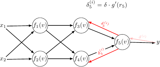
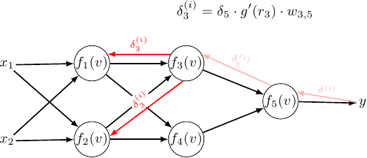
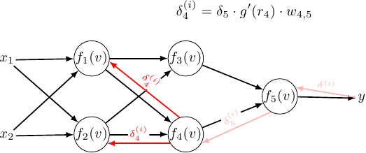
So for the second hidden layer:

\[\delta_3^{(i)} = \delta^{(i)} \cdot g'(r_5) \cdot w_{3,5}\] \[\delta_4^{(i)} = \delta^{(i)} \cdot g'(r_5) \cdot w_{4,5}\] \[\displaystyle w_{1,3}^{(l + 1)} = w_{1,3}^{(l)} - h \cdot \sum \limits_{i = 1}^{M} {\color{red} \delta_3^{(i)}} \cdot {\color{green} g'(r_3) } \cdot {\color{blue} g(r_1) }\] \[\displaystyle w_{1,4}^{(l + 1)} = w_{1,4}^{(l)} - h \cdot \sum \limits_{i = 1}^{M} {\color{red} \delta_4^{(i)}} \cdot {\color{green} g'(r_4) } \cdot {\color{blue} g(r_1) }\] \[\displaystyle w_{2,3}^{(l + 1)} = w_{2,3}^{(l)} - h \cdot \sum \limits_{i = 1}^{M} {\color{red} \delta_3^{(i)}} \cdot {\color{green} g'(r_3) } \cdot {\color{blue} g(r_2) }\] \[\displaystyle w_{2,4}^{(l + 1)} = w_{2,4}^{(l)} - h \cdot \sum \limits_{i = 1}^{M} {\color{red} \delta_4^{(i)}} \cdot {\color{green} g'(r_4) } \cdot {\color{blue} g(r_2) }\]

Does it hold for the first hidden layer?:

\[\displaystyle \delta_1^{(i)} = \delta_3^{(i)} \cdot g'(r_3) \cdot w_{1,3} + \delta_4^{(i)} \cdot g'(r_4) \cdot w_{1,4}\] \[\displaystyle w_{x_1,1}^{(l+1)} = w_{x_1,1}^{(l)} - h \sum_{i = 1}^{M} {\color{red} \delta_1^{(i)}} \cdot {\color{green} g'(r_4) } \cdot {\color{blue} x_1 } =\] \[\displaystyle w_{x_1,1}^{(l+1)} = w_{x_1,1}^{(l)} - h \sum_{i = 1}^{M} \left( \delta_3^{(i)} \cdot g'(r_3) \cdot w_{1,3} + \delta_4^{(i)} \cdot g'(r_4) \cdot w_{1,4} \right) g'(r_4) \cdot x_1\]

I’ll try to tidy up the expression in parenthesis:

\[\displaystyle \left( \delta_3^{(i)} \cdot g'(r_3) \cdot w_{1,3} + \delta_4^{(i)} \cdot g'(r_4) \cdot w_{1,4} \right) =\] \[\displaystyle \left( \delta^{(i)} g'(r_5) w_{3,5} g'(r_3) w_{1,3} + \delta^{(i)} g'(r_5) w_{4,5} g'(r_4) w_{1,4} \right) =\] \[\displaystyle \delta^{(i)} g'(r_5) \left( w_{3,5} g'(r_3) w_{1,3} + w_{4,5} g'(r_4) w_{1,4} \right)\]

Substituting it back:

\[\displaystyle w_{x_1,1}^{(l+1)} = w_{x_1,1}^{(l)} - h \sum_{i = 1}^{M} \delta^{(i)} g'(r_5) g'(r_4) \cdot x_1 \left( w_{3,5} g'(r_3) w_{1,3} + w_{4,5} g'(r_4) w_{1,4} \right)\]

Which is the same term we came up with previously, when we derived it explicitly.

Summary

To sum up:

• The gist of the weight update algorithm is error backpropagation.
• The error signal “travels” from the output layer to the input layerj
• The weights influence the error by some degree, and that weight must be taken into account when propagating the error.

And finally, some pictures. I’ve highlighted how the error signal propagates through the network, and how the previous errors contributed to the current error: