While at university, for a graphics processing class as an assignment I chose to implement the seam carving algorithm.

This rescaling/refocusing algorithm works by iteratively calculating the finite difference of an image in either \(x\) or \(y\) dimension, finding a seam (connected path of pixel differences) with the lowest “energy” (sum) and removing the seam.

To get back an image after removing the seam you need to reintegrate the finite differences to obtain the rescaled image. This algorithm led me into the rabbit hole of Poisson image editing but unfortunately at the time it was hard to find or implement a Poisson solver in java so my seam carving implementation simply removed pixels from the source image and applied a blur around the removed seams without reintegrating.

But the thought of implementing a Poisson solver has stuck with me and nowadays we can use SIMD instructions from within the JVM itself so reasonable performance should be achievable.

The code used to generate the images found in this article can be found here. I won’t go much into details of the implementation so if you’re fine with reading a little bit of Scala and have some background in image processing going through blog post should be possible.

The gradient domain

When evaluating the finite differences of some image \(I\) in \(x\) or \(y\) dimensions we get two matrices \(D_x(I)\) and \(D_y(I)\). Where:

\(D_x(I)_{x,y} = I_{x,y} - I_{x-1,y} \quad \forall x = 1 \ldots \text{width}(I) - 1, y = 0 \ldots \text{height}(I) - 1\) \(D_y(I)_{x,y} = I_{x,y} - I_{x,y-1} \quad \forall x = 0 \ldots \text{width}(I) - 1, y = 1 \ldots \text{height}(I) - 1\)

When operating on the finite difference matrices, by say cutting out a vertical seam, and reintegrating both finite difference matrices the resulting image matrices might produce two images that don’t 100% agree anymore.

Finding an image that minimizes the least square error between the two gradient is equivalent to solving the Poisson’s equation¹:

\[\nabla^2 u = D_x(D_x(I)) + D_y(D_y(I))\]

And I will refer to the rhs of the equation as the laplacian of the image.

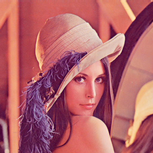
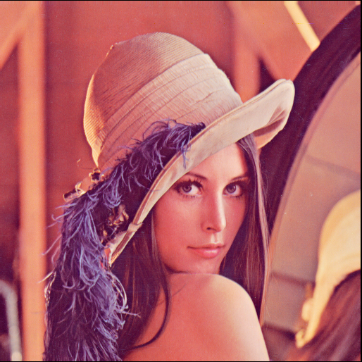
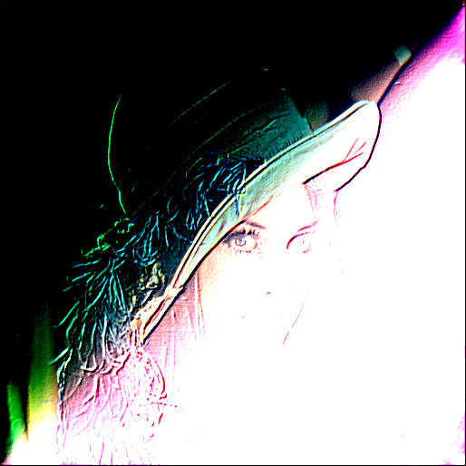
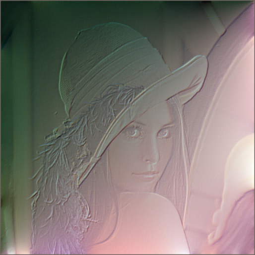
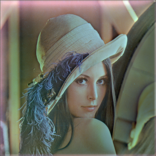
To illustrate how a laplacian “looks” I will use two images.

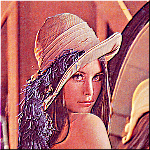
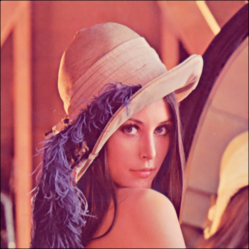
The “standard” test image Lenna:

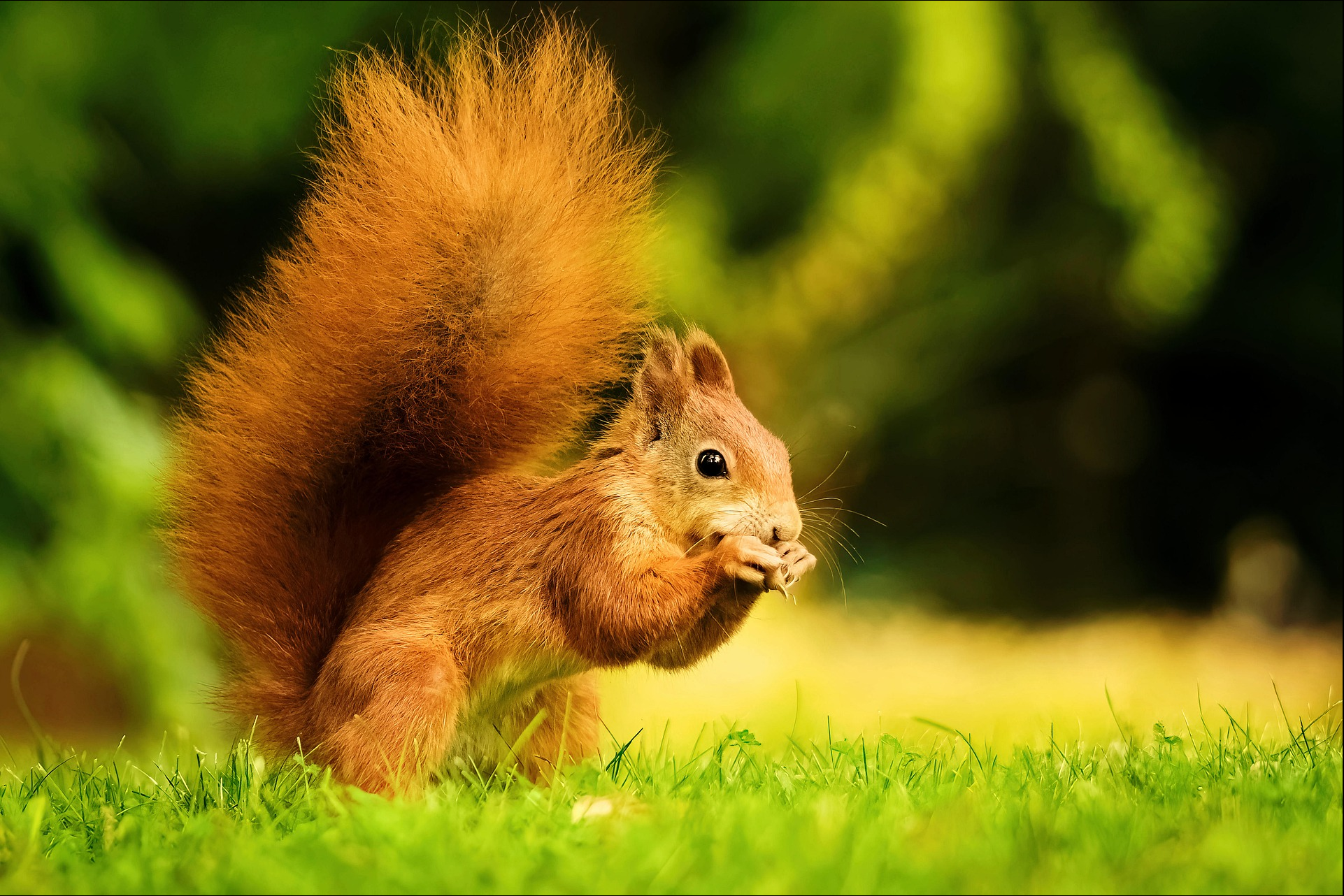
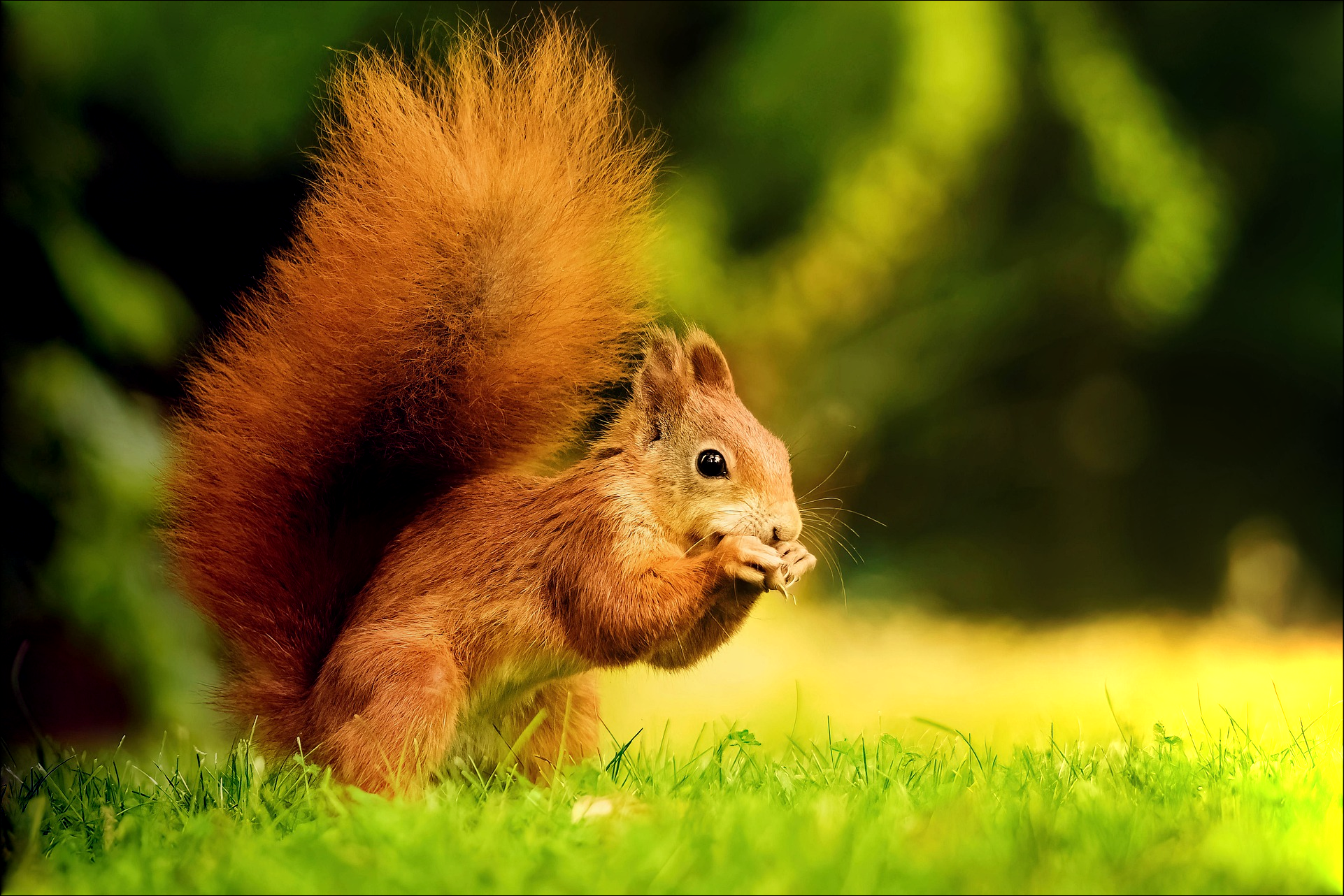
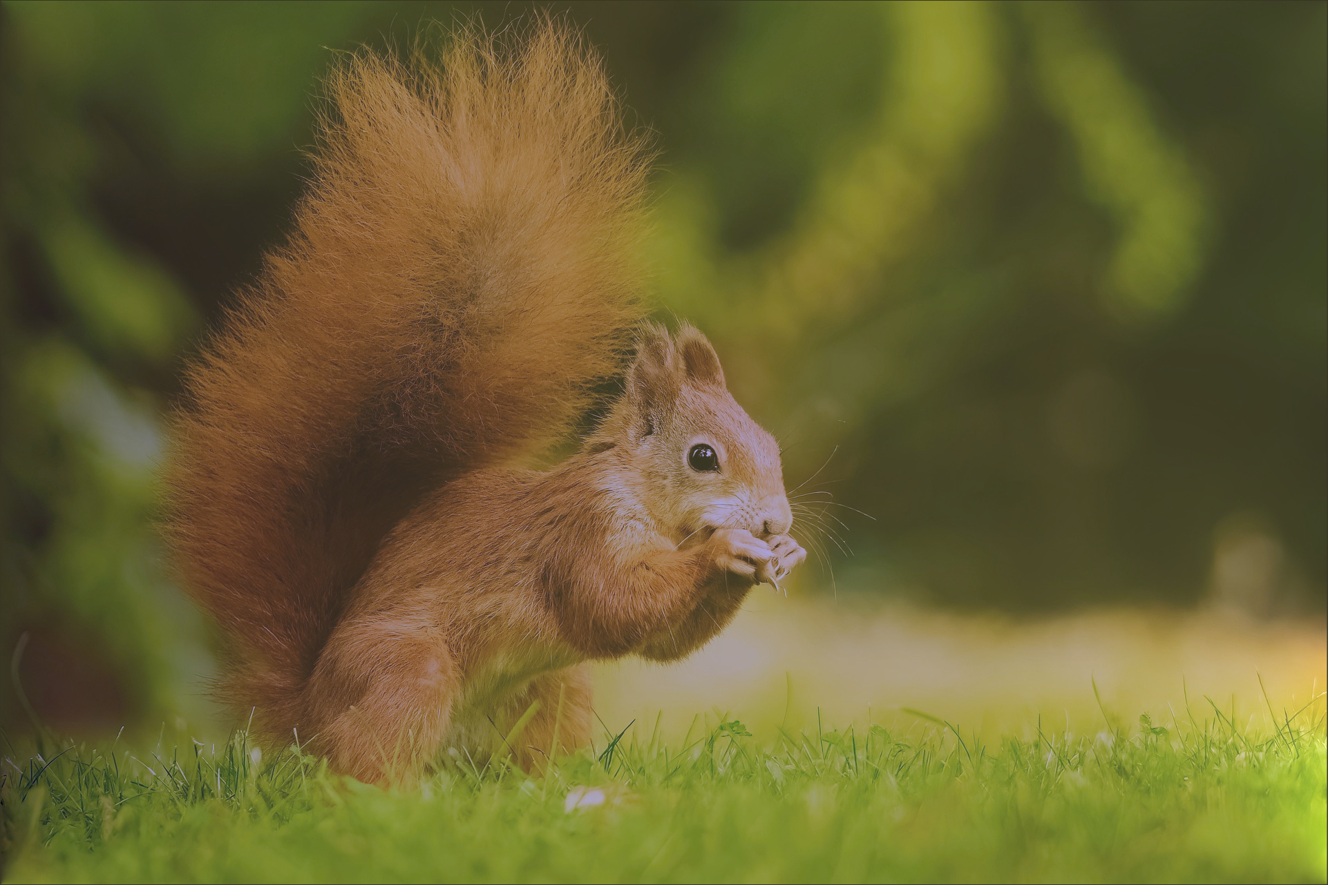
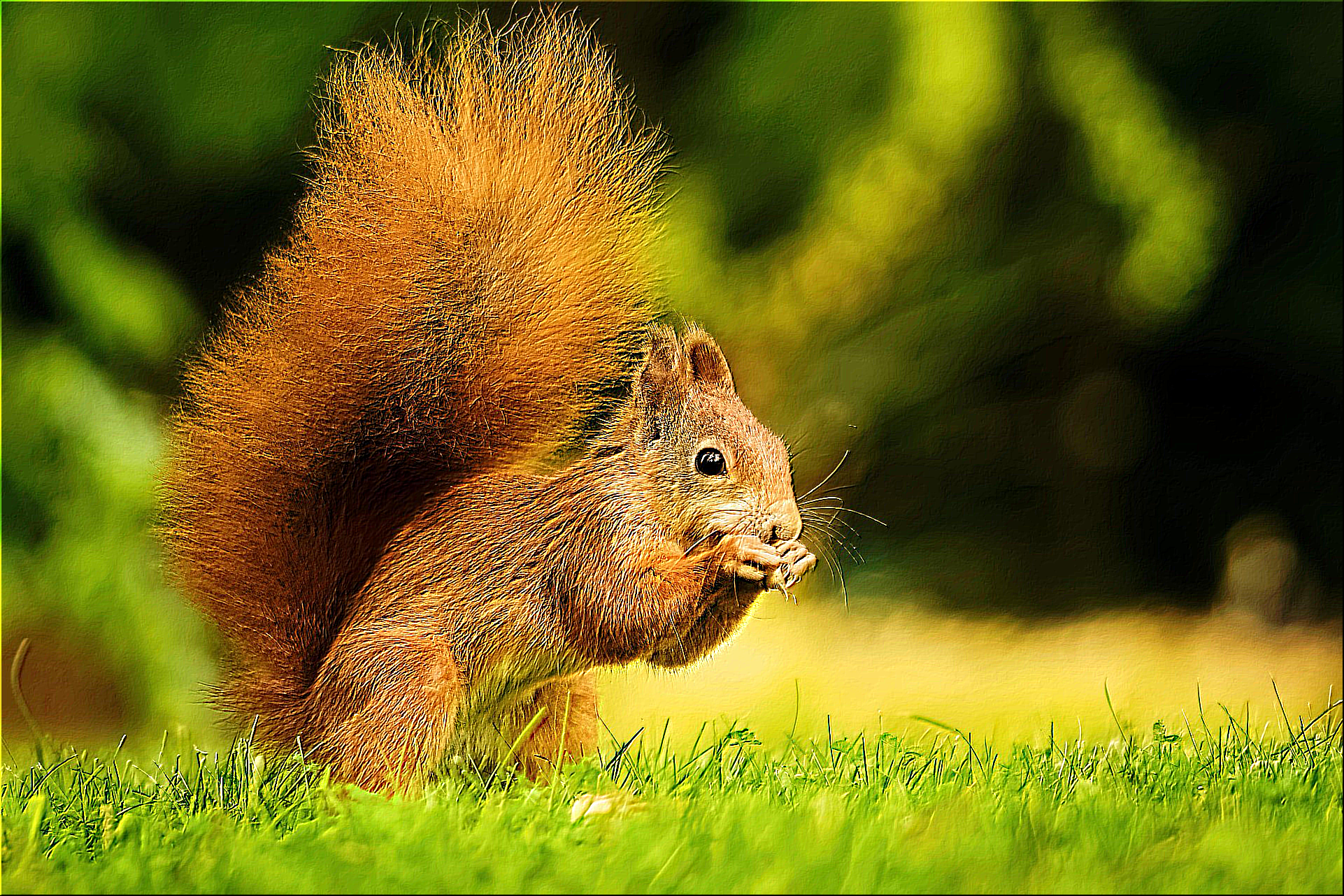
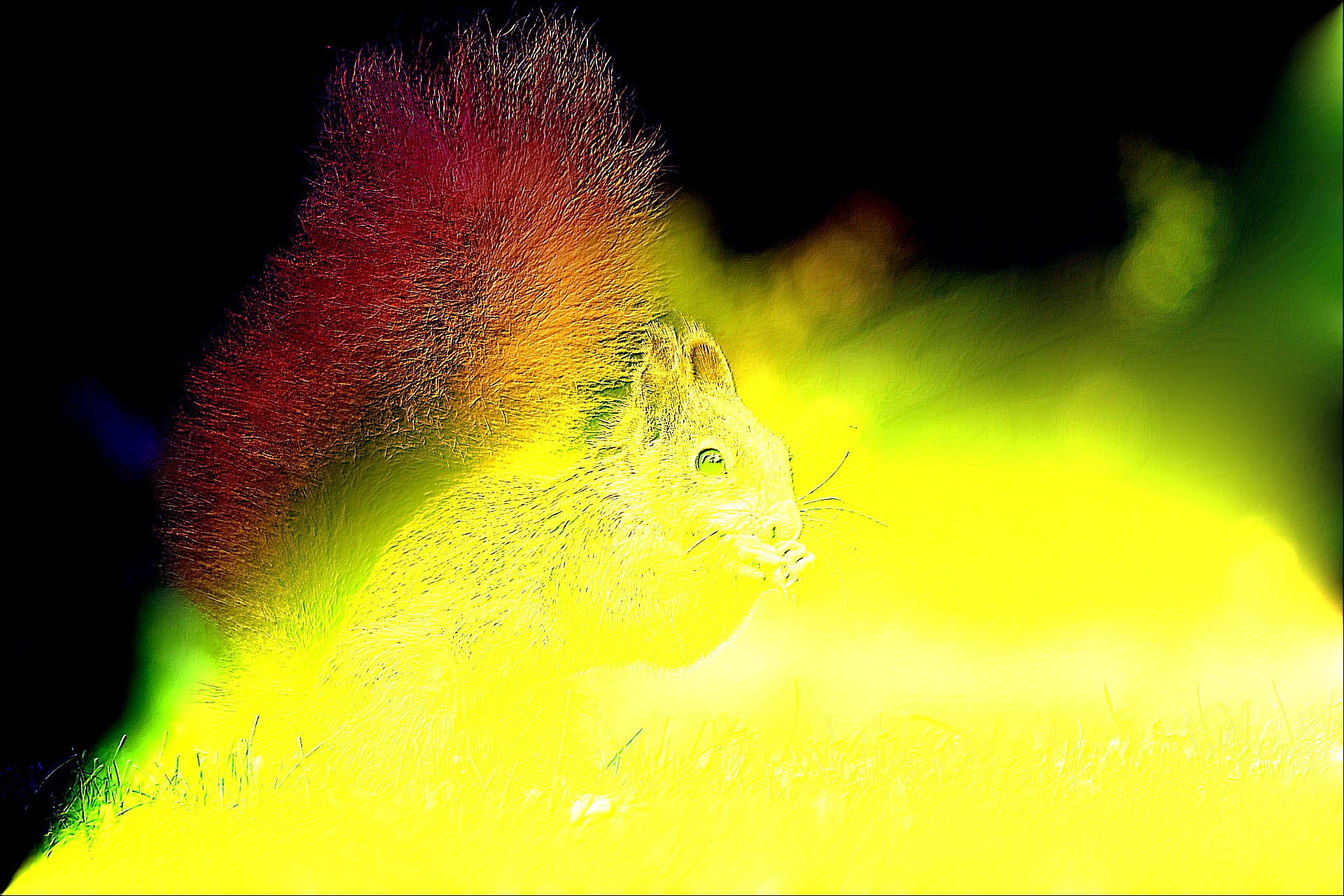
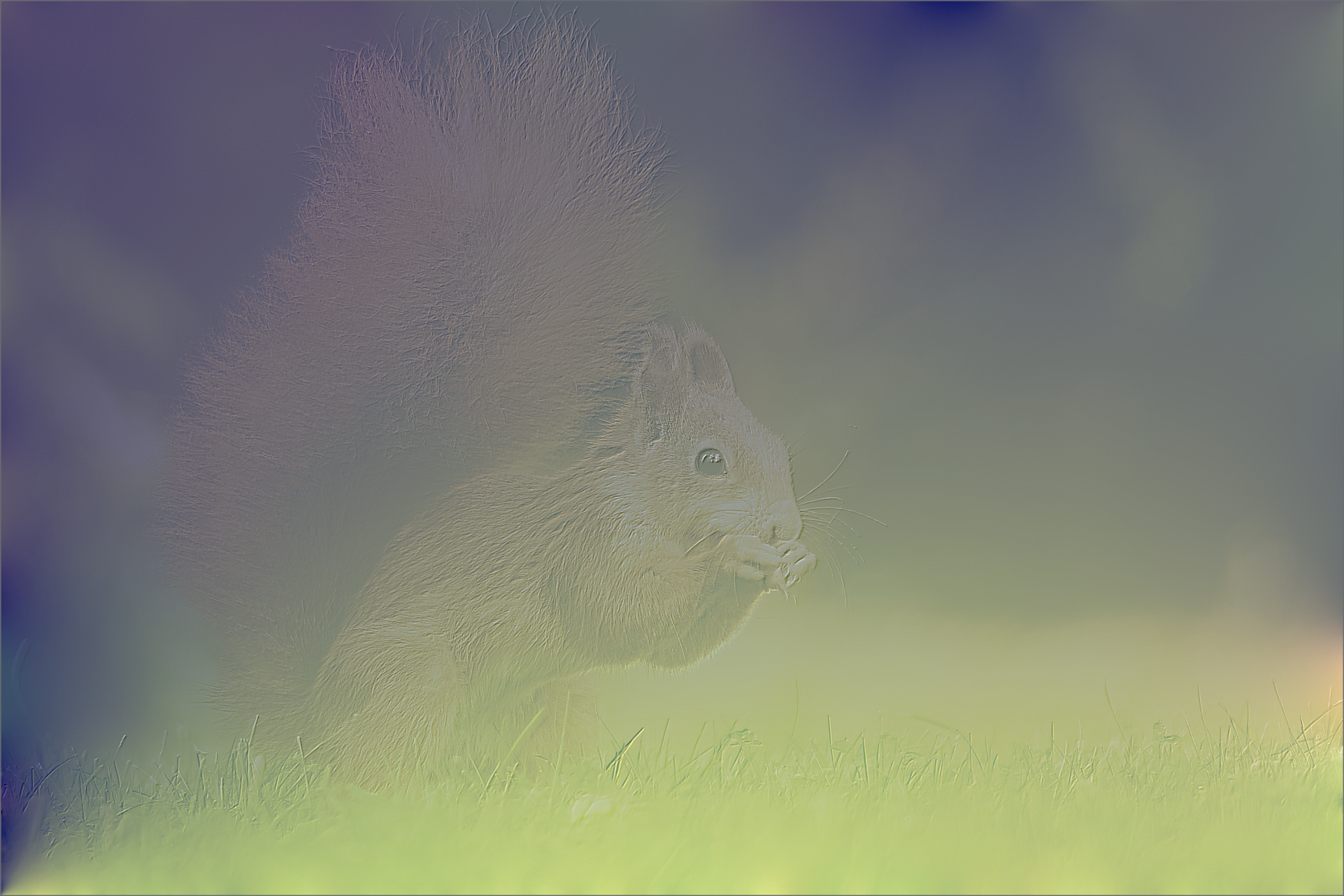
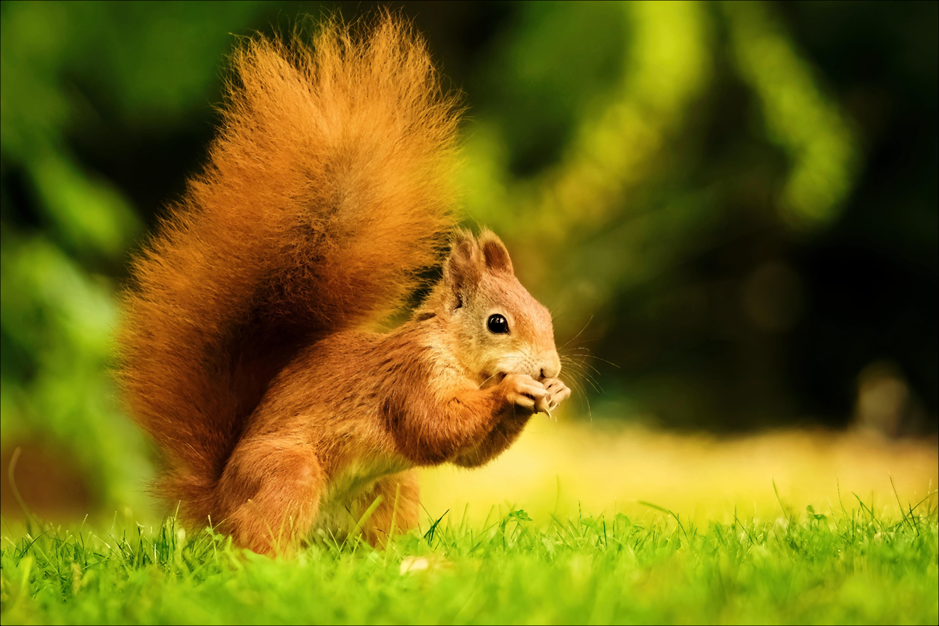
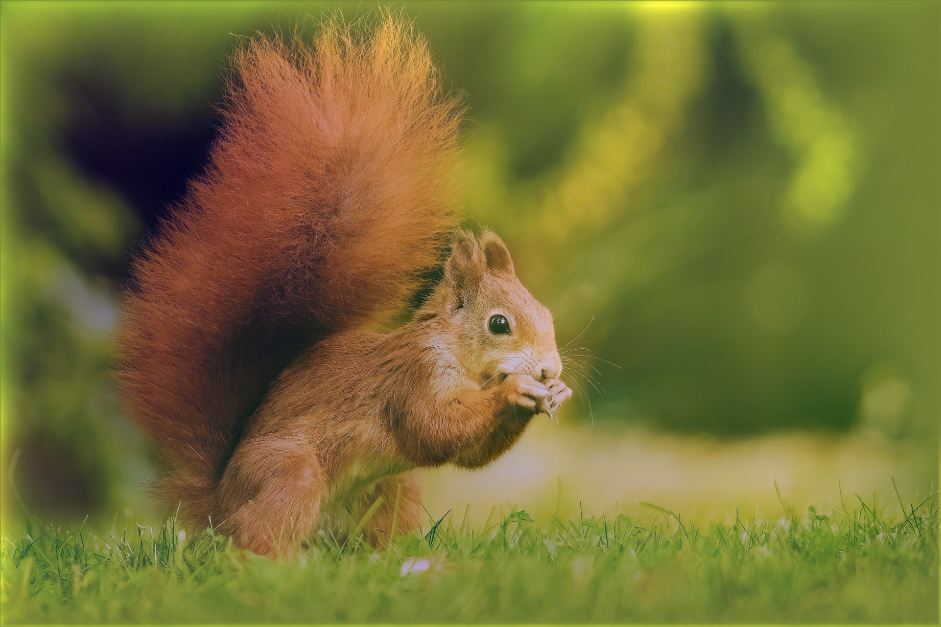
A squirrel image I got from pixabay:

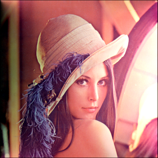
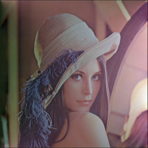
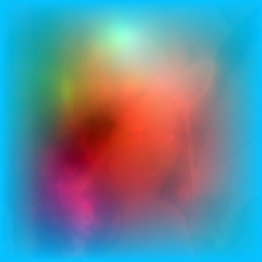
After renormalizing² the values to lie on \([0, 1]\)the respective laplacians of the b channel of each image looks like this (click on the full resolution image to see the details).

The white values correspond to positive peaks of the laplacian (large positive changes in either \(x\) or \(y\)) and black to to negative peaks of the laplacian (large negative changes in either \(x\) or \(y\)).

Writing the Poisson Solver

There are many algorithms that find the solution of Poisson’s equation but precise methods involve inverting large matrices which is never fun.

On the other hand, relaxation methods are often easy to implement and have low memory requirements but operate on a local neighborhoods and their convergence is very slow.

Fortunately, there exists an algorithm (called the multigrid algorithm) which recursively scales down the laplacian and finds a “coarse” solution³ to the problem that gets upscaled as a starting approximations of the “current” level.

This makes the convergence very fast as large areas in the original-scale solution are populated by good guesses via successive approximations from coarser scales which compansates for the local nature of the relaxation methods.

Wikipedia’s description of the algorithm is decent… if you understand what smoothing, restriction and prolongation is and how to calculate the residual.

I won’t go into detail about the multigrid algorithm itself but when implementing the algorithm the best resources⁴ I stumbled upon were:

• Multigrid method from MIT Computational Thinking course for the motivation and an easy to follow multigrid-like algorithm.
• Iterative methods and Multigrid from Qiqi Wang’s lectures which describe the deriviations of the finite difference method in an approchable way.
• Multigrid Methods with Repa which has a very clear implementation of the multigrid method itself and following along the code helped me track down some stupid errors in my implementation.

A small note on boundary-values

The laplacian doesn’t describe an unique image - the simple intuition behind this fact is that the definition of finite difference encodes differences between pixel rows (\(D_x(I)\)) and pixel columns (\(D_y(I)\)) and that difference is missing for the last row/column. Hence to recover the original image from the whole we also need to provide the pixel values of the last row and column to the solver as an initial guess.

In my implementation I chose to tackle boundary values in two ways:

• always use the entire 1-pixel border for boundary values and not only the last row/column⁵
• before calculating the laplacian artifically expand the input images by 1 black pixel (i.e. 0.0 values in each channel) in each direction.

Implementation

Individual steps that need to be done to fully implement the multigrid solver:

1. Writing a relaxation method and residual calculation.
2. Implementing the restriction (fine grid -> coarser grid) and prolongation (coarse grid -> finer grid) operators taking care of properly treaing boundary conditions.
3. Implementing the recursive multigrid method
4. Optimizing (vectorization)

In my case I started with a Jacobi solver but settled experimentally on a Jacobi with successive over-relaxation. That was a small change to implement and it increased the convergence rate significantly.

Both restriction and interpolation operators are implemented via bilinear scaling. For the restriction operator, since I know that my initial boundary conditions will always be at the pixel borders when scaling down the laplacian I always leave a 1 pixel boundary intact⁶. The prolongation operator is straight up bilinear scaling but applying the residual error I, additionally, restore the boundary conditions.

The biggest speed up was related to vectorizing the Jacobi iteration. I also tried parallelizing the Jacobi iteration but apparently the overhead of naive parallelization is too much for any speedup to be observable, hence the only parallelism in the final implementation is related to solving each channel of the image in parallel.

Playing Around in the Gradient Domain

To get a feel for the Poisson editing I decided to implement a couple of simple graphical operations.

One of the surprises was that convolutions in the Poisson domain give exactly the same results as in the image domain!

At first this seemed unintuitive, as my naive expectation was that any operation in the Poisson domain would cause exaggerated changes in the image domain.

But since operating in the Poisson domain is the same as operating on (sums of) image differences it stands to a reason that any operator that multiplies differences by a factor would produce the same laplacians as the image multiplied by a factor:

\[\alpha D_x(I)_{x,y} = \alpha (I_{x,y} - I_{x-1,y}) = \alpha I_{x,y} - \alpha I_{x - 1, y}\]

hence

\[\alpha D_x(I) = D_x(\alpha I)\]

Similarly, the sum of arbitrary finite differences is the same as the sum of the differences of the images at those positions.

\[D_x(I)_{x,y} + D_x(I)_{x', y'} = I_{x,y} - I_{x-1,y} + I_{x',y'} - I_{x'-1,y'}\]

and since convolution by definition is just local sums and multiplications this explains the equivalence.

This obviously doesn’t apply to non-linear transformations like convolutions with non-symmetric kernels⁷ or any other non linear operation

Compare the results of these nonlinear operations.

Translation convolution

Convolving an image by this kernel

\[\left [ \begin{array}{ccc} 0 & 0 & 0 \\ 1 & 0 & 0 \\ 0 & 0 & 0 \end{array} \right ]\]

which simply moves the image by 1 pixel to the right:

• Convolution the poisson domain:

• Convolution with the kernel in the poisson domain with normalization (note blue/green tint in the lower left of the image)

• Squirrel: convolution in the image domain

• Squirrel: convolution in the poisson domain (note deepend shadows in the left part of the image)

• Squirrel: convolution in the poisson domain normalized

Emboss

Emboss is defined as the kernel:

\[\left [ \begin{array}{ccc} 2 & 1 & 0 \\ 1 & 1 & -1 \\ 0 & -1 & -2 \end{array} \right ]\]

which when applied in the image domain applies an embossing effect.

• Lenna with the embossing effect:

• Emboss effect in the poisson domain:

• Emboss effect in the poisson domain normalized:

• Squirrel: emboss effect in the image domain

• Squirrel: emboss effect in the poisson domain

• Squirrel: emboss effect in the poisson domain normalized

Median filter

The median filter is a classic image processing algorithm which like convolution operates on a window but the convolutional operation is replaced by taking the median of the windowed pixels.

In the image domain this is usually used to de-noise an image, although it also usually gives an image a fake plastic-like look, especially on larger kernels.

Applying the median filter in the laplace domain creates an image that’s heavily oversaturated but after applying normalization the filter seems to catch aspects of the image’s saliency

• Lenna median filter:

• Emboss effect in the poisson domain normalized:

• Squirrel: median effect in the image domain

• Squirrel: median effect in the poisson domain normalized

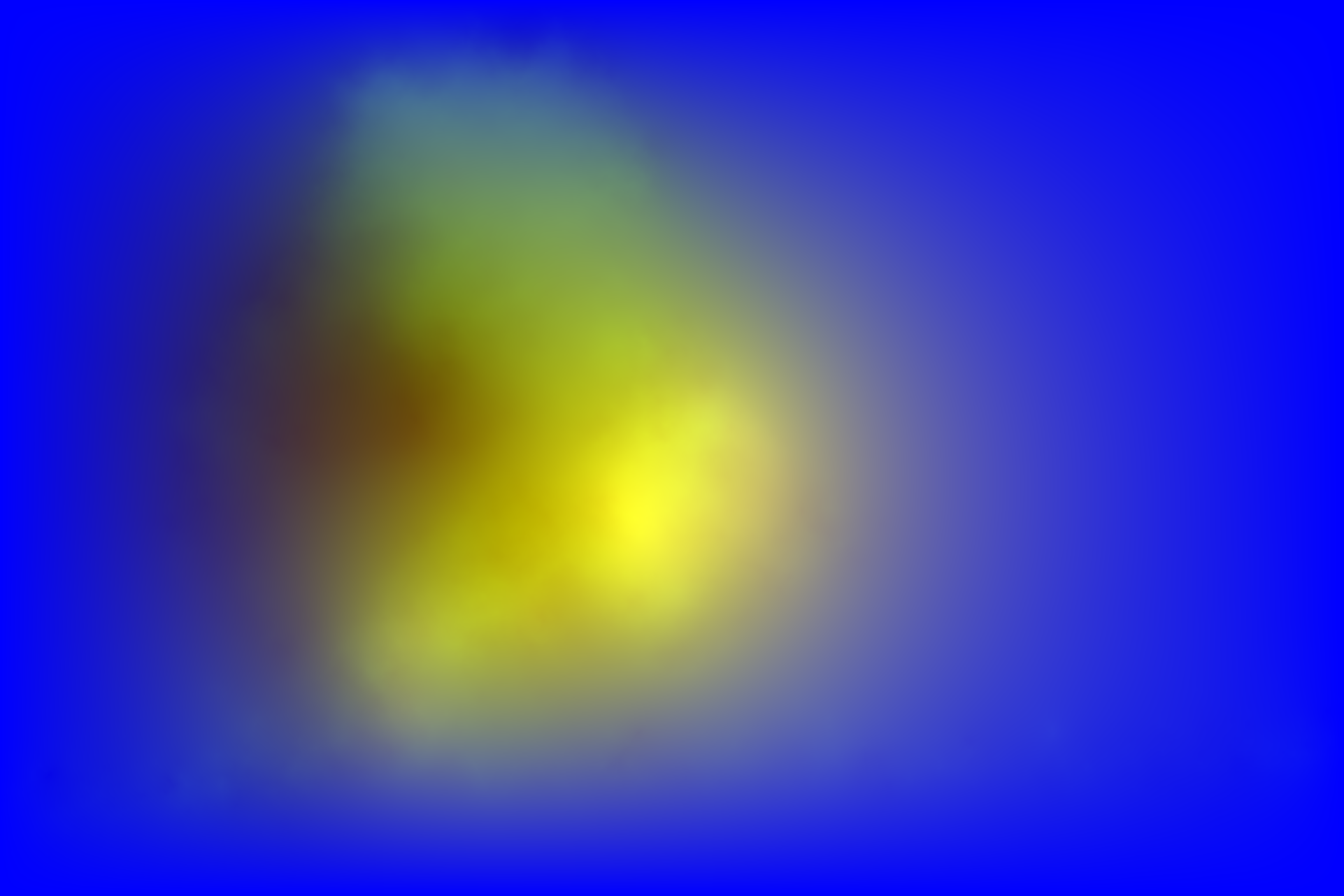
Image blending

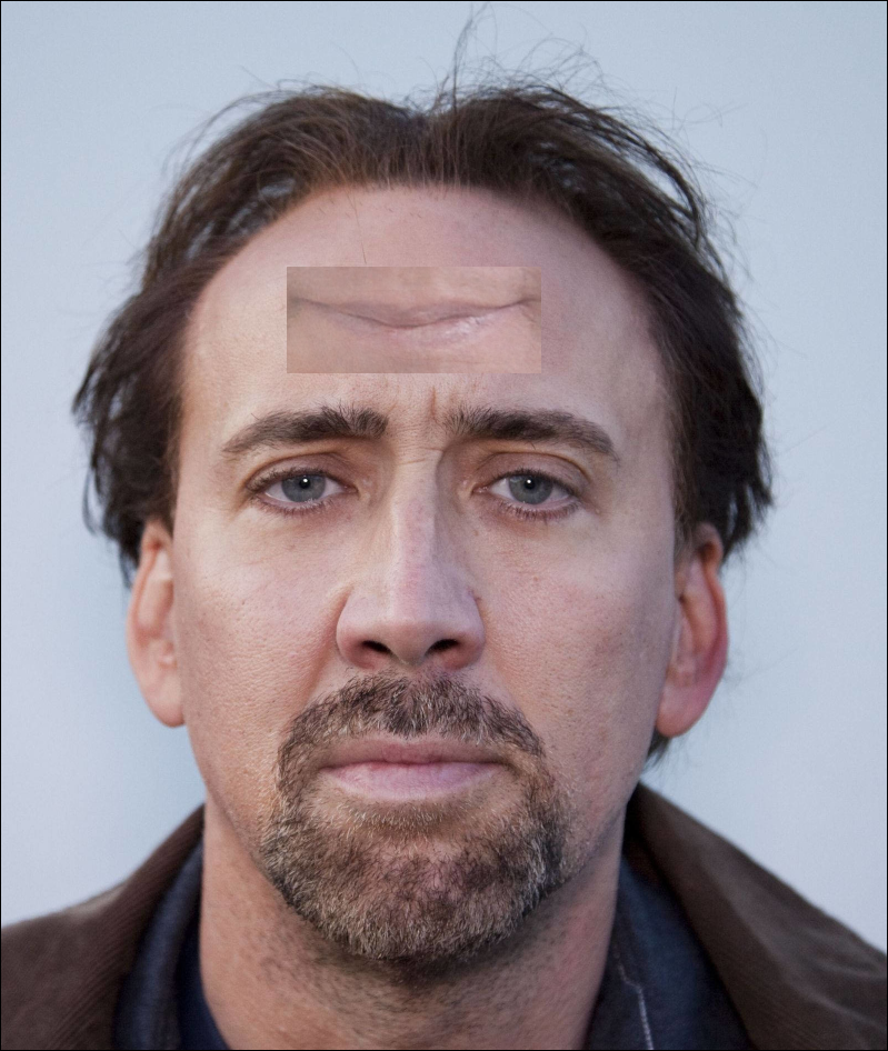
One famous use of poisson image editing is image blending:

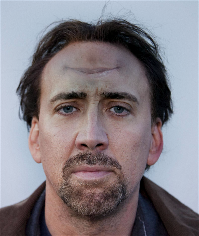
This image was produced by blending a region from a region of a picture of the actor John Travolta onto the forhead region in the Nicolas Cage image.

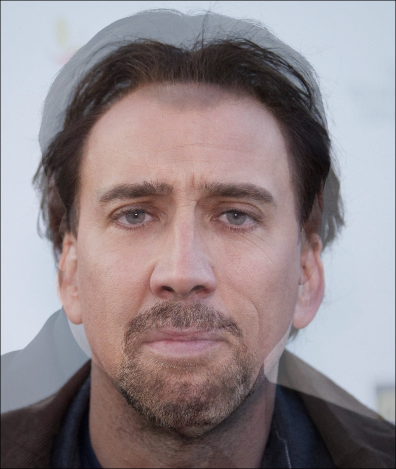
• Nicolas cage image

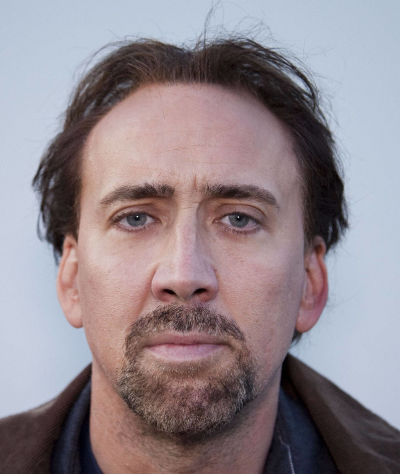
• John Travolta image

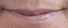
• cropped mouth region:

The blending was done by averaging the laplacian from both images in the pasted region.

By comparison, doing this averaging in the image domain makes for a less convincing image blending:

Knowing that multiplying and summing image differences is an operation neutral to the poisson transform, it should⁸ come as no suprise that blending entire images this way will give the same results as blending in the image domain:

Final thoughts

Since implementing a poisson solver was on my TODO-list for some time now, I finally feel a sense of accomplishment.

Speed-wise with the default setting (50 iterations of the multigrid algorithm, 20 pre-smoothing operations, 60 post-smoothing) it takes over 50 seconds to reintegrate the laplacian of the squirrel image (1920x1080).

Sensible results can be obtained even faster: with just 2 multigrid, 2 pre-smoothing and 4 post-smoothing operations a low quality approximation of the final image can be obtained under a second.

Thanks to iterative nature of Jacobi/multigrid method implementing this would be good enough for real time applications if the updates were propagated often enough. This could be further supplemented by a proper multithreading implementation of the multigrid algorithm.

I also really want to try my hand in implementing an alternative algorithm which claims even faster speeds but I stumbled upon it relatively late when writing this article.

Due to sensitivity to initial conditions, operations on the poisson domain aren’t overly intuitive but even observing failure cases makes me want to try out implementing more complicated filters a la Gradientshop.

Another thing I really wanted to try is generating images from samples like in Scene Completion Using Millions of Photographs by Hays and Efros albeit with a simpler models e.g. Markov chains.

Footnotes